10 Simple Bayesian Nonlinear Regression
1 Introduction
An example of simple nonlinear regression is discussed in section C of NONMEM Users Guide, Part I. This example is continued in this section in order to illustrate the discussion concerning constraints given in section B and in order to illustrate several additional NONMEM features. The first additional feature to be illustrated is the Theta Constraint Option, by which one may exercise some control over the way the constraints on the theta elements (see section C.4 of NONMEM Users Guide, Part I) are implemented inside the NONMEM program itself. The second additional feature gives the user the option to add a forty-five degree line onto a scatterplot. This can be useful when, for example, in a simple nonlinear regression, predictions are plotted against observations. The last additional feature gives the user the option to modify the way in which the objective function is computed (while the statistical model itself remains fixed); this involves use of a user-supplied subroutine, CRIT. The basic computation that is presented here, one of a simple Bayesian nonlinear regression, does not, however, depend on the presence of any of the additional features just mentioned, and it may be carried out as illustrated below with only NONMEM features described in NONMEM users Guide, Part I, and constraints on omega as discussed in section B of this document.
In Section 10.2 the theoretical aspects of the example are discussed. In Section 10.3, implementation of the example is discussed. The three additional features that are mentioned above are discussed in Section 10.4 through Section 10.6. The reader can go immediately to these sections if he wishes only to review the use of these additional features.
2 An Example
We continue the example of section C in the NONMEM Users Guide, Part I. First, we reparametrize the function, \(f\), as follows
\[ f(\theta_1, \theta_2, \theta_3, X_1, X_2) = \frac{\theta_1 \theta_2 X_1}{\theta_3 (\theta_1 - \theta_2)} \left(\exp(-\theta_2 X_2) - \exp(-\theta_1 X_2)\right) \]
In words, we have redefined \(\theta_3\) to be the product of \(\theta_2\) and the original \(\theta_3\). In pharmacokinetic language, \(\theta_3\) now denotes drug clearance, where before it denoted volume.
The data in the old example are ten plasma concentrations from a single subject, S, from a certain population. The (true) value of \(\theta = (\theta_1, \theta_2, \theta_3)\) varies from subject to subject within this population. Although in this new example we are again interested in the (true) value of \(\theta\) for S, here we shall consider an estimate of this value that is based on knowledge of how \(\theta\) varies in the population, in addition to the plasma concentration data from S. The population itself has been studied by measuring plasma concentrations from each of a sample of twelve subjects chosen from the population. This larger data set was used in the example in section F of the NONMEM Users Guide, Part I, wherein estimates, \(\bar{\theta} = (\bar{\theta}_1, \bar{\theta}_2, \bar{\theta}_3)\) and C, of the mean and covariance, respectively, of \(\theta\) in the population were obtained. Actually, \(\bar{\theta}_3\) was obtained for each of a family of subpopulations obtained by “stratifying” the population by body weight. The estimate, \(\bar{\theta}_3\) is characterized then as a function of weight. The relationship of \(\bar{\theta}_3\) to weight is a simple proportional one. Since the weight of S, in particular, is 72.4, \(\bar{\theta}_3\) for the particular subpopulation of interest is given by the proportionality constant, .0363, times 72.4, i.e. 2.63. On the other hand, in the analysis of the population data, \(\theta\) was assumed to have homogeneous covariance in the population. Another important population parameter was estimated in the example of section F of NONMEM Users Guide, Part I. This parameter (denoted in that example by \(\Sigma\)) is the variance of the plasma concentrations from any population member, given that member’s value of \(\theta\), and it is independent of \(\theta\). Denote its estimate by \(\sigma^2\).
Consequently, in addition to the ten measurements from S there are three other measurements from the population that have information about \(\theta\) for S, namely: \(\bar{\theta}_1\), \(\bar{\theta}_2\), and \(\bar{\theta}_3\). More precisely,
\[\bar{\theta}_i = \theta_i + \eta_{io} \quad i = 1, 2, 3\]
where
\[E(\eta_{10}, \eta_{20}, \eta_{30}) = 0\]
\[\mathrm{Cov}(\eta_{10}, \eta_{20}, \eta_{30}) = C.\]
(Of course, C is only an estimate of the covariance, and the assumption that the expectation is 0 is compromised by the fact that the \(\bar{\theta}_i\) are only estimates of the true means of the \(\theta_i\). However, some people feel that often one is better off using some prior (population) information about the unknown parameter one is trying to estimate, rather than none at all, even if this information is not very precise.) Combining this model with the model for the ten plasma concentrations, we obtain
\[Y_{io} = \theta_i + \eta_{io} \quad i = 1, 2, 3\]
\[Y_{1j} = f(\theta_1, \theta_2, \theta_3, X_{1j}, X_{2j}) + \eta_{4j} \quad j = 1, 2, 3, \ldots, 10\]
\[E(\eta_{1j}, \eta_{2j}, \eta_{3j}, \eta_{4j}) = 0 \quad j = 0, 1, 2, \ldots, 10\]
\[\mathrm{Cov}(\eta_{1j}, \eta_{2j}, \eta_{3j}, \eta_{4j}) = \begin{pmatrix} C & 0 \\ 0 & \sigma^2 \end{pmatrix} \quad j = 0, 1, 2, \ldots, 10\]
Here, \(Y_{io} = \bar{\theta}\) and the \(Y_{1j}\) are the ten plasma concentrations. This is an example of a model with equivalently nested random effects and NONMEM may be used. (See section D.6 of NONMEM Users Guide, Part I.) Of course, one must be able to constrain the covariance matrix of the \(\eta_{ki}\) as specified above. This, though, is the major point of this example, and the set up for NONMEM is described in the next section.
The (default) objective function for this particular model is
\[O(\theta_1, \theta_2, \theta_3) = Y_0 C^{-1} Y_0^T + \sum_{j=1}^{10} (Y_{1j} - f(\theta_1, \theta_2, \theta_3, X_{1j}, X_{2j}))^2 / \sigma^2\]
plus another (log) term that is independent of \(\theta\), as may be seen by regarding the objective function for the general model with equivalently nested random effects. Here \(Y_0 = (Y_{10}, Y_{20}, Y_{30})\). Note that \(\sigma^2\) is not an argument of this function, in contrast with the situation in the old example, since in this new example we assume it to be a known constant. Instead of viewing the population information as giving rise to a model with equivalently nested random effects, one may take another view that leads to the same objective function. Assume that \(\theta\) is normally distributed in the population with mean \(\bar{\theta}\) and covariance C. This multivariate distribution is taken as a prior distribution on \(\theta\) for S. Assume also that the conditional distribution of \(Y_{1j}\), given \(\theta\), is normal with mean \(f(\theta_1, \theta_2, \theta_3, X_{1j}, X_{2j})\) and variance \(\sigma^2\). Then using Bayes formula (Rao 1973, 334) the negative log of the posterior density of \(\theta\), may be seen to equal the above objective function, again up to a term independent of \(\theta\). From this point of view the estimate of \(\theta\) obtained from minimizing this objective function is the mode of the posterior distribution.
3 Implementation of the Example
A code for PRED is given in Figure 1. There it may be seen that an additional data item is used to determine whether the DV data item is an observed concentration or an element of \(\bar{\theta}\). If the value of this data item is zero, the DV data item is an observed concentration; if it is i, the DV data item is \(\bar{\theta}_i\).
The problem specification is given in Figure 2. Upon examining the data, one sees that a fifth data item also has been added. This is the ID data item. It is there because the \(\eta_k\) are random individual effects.
In this example the block set partition for omega has two block sets, each of these block sets has a single block, and the two blocks have dimension 3 and 1. This is reflected in fields 6 and 7 of the initial STRUCTURE record and in the STRUCTURE record for omega. Note also that there is a one in position 8 of both BLOCK SET records, thus constraining the two blocks to C and \(\sigma^2\), respectively, the values of which are specified on these records. There is no sigma matrix.
There is a two in field 5 of the initial STRUCTURE record, and there is a one in field 6 of the last SCATTERPLOT record. These specifications are discussed in Section 10.4 and Section 10.5.
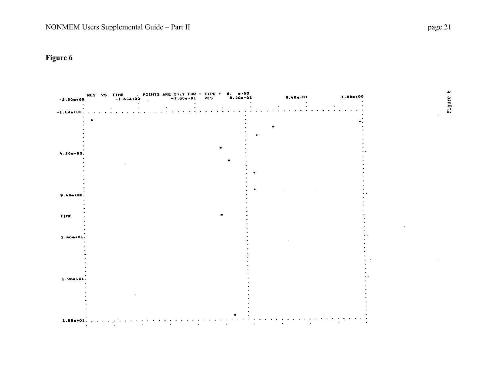
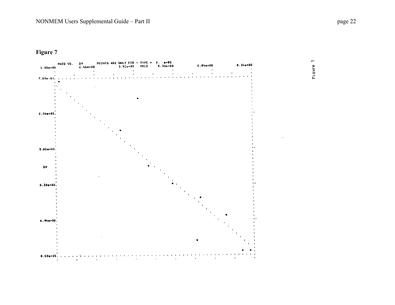
Some output is shown in Figure 3, Figure 4, Figure 5, Figure 6, Figure 7. The summary of the problem specification is given in Figure 3, Figure 4. Note that there the block diagonal form of omega is schematically displayed as a patterned lower triangular matrix, and that the initial estimate of omega is displayed by giving the initial estimate of each of the two blocks separately. There is also an indication there that each block is constrained, or fixed, to its initial estimate. The final estimate is shown in Figure 5. The final estimate of omega is, of course, equal to the initial estimate. Some of the scatterplots are displayed in Figure 6, Figure 7. These are discussed in Section 10.5.
4 The Theta Constraint Option (Obsolete)
An element, \(\theta_m\), of theta may be bounded above and below by different finite numbers, a and b, respectively. This is accomplished by i) taking a function, T, defined on all real numbers, and whose range is the interval (b, a), ii) defining a new unconstrained parameter, \(\varphi_m\) satisfying
\[\theta_m = T(\varphi_m)\]
and iii) reparametrizing the functions \(f\), \(g_{kij}\) and \(h_{lij}\) in terms of \(\varphi_m\). All the user need do for these steps to be carried out is to use fields 4 and 5 of the initial STRUCTURE record and the LOWER and UPPER records as described in section C of NONMEM Users Guide, Part I. The value one placed in both fields 4 and 5 of the initial STRUCTURE record satisfies the requirement for that record, and all relevant examples in NONMEM Users Guide, Part I, show the value one in these fields. In this case T is given by
\[T(x) = b + (a - b) \sin^2(x)\]
A message that the arcsin transform is used appears on the summary of the problem specification: the arcsin is, of course the “inverse” of the sin function. The Theta Constraint Option allows the user to choose an alternative form for T. If the value two is placed in field 5 (see Figure 2), rather than one, T is given by
\[T(x) = b + (a - b) \frac{\exp(x)}{1 + \exp(x)}\]
A message that the logit transform is used appears on the summary of the problem specification; see Figure 3. The logit is, of course, the inverse of the function:
\[x \to \frac{\exp(x)}{1 + \exp(x)}\]
Note that whatever choice for T is made, it applies to all elements of theta bounded above and below by different finite numbers. The complete format of the initial STRUCTURE record is given in Table 1.
| Field no. | Value | Function |
|---|---|---|
| 1 | between 0 & 70 | length of theta vector |
| 2 | between 0 & 70 | length eta vector |
| 3 | between 0 & 70 | length of epsilon vector |
| 4 | blank | |
| 5 | blank | |
| 6 | 0 or blank | omega constrained with a block set partition |
| 6 | 1 | omega constrained to be of simple diagonal form |
| 7 | 0 or blank between 1 & 70 | only if field 6 has value 1 number of block sets for omega |
| If the length of the epsilon vector is 0, the following fields may be ignored. | ||
| 8 | 0 or blank | sigma constrained with a block set partition |
| 8 | 1 | sigma constrained to be of simple diagonal form |
| 9 | 0 or blank between 1 & 70 | only if field 8 has value 1 number of block sets for sigma |
5 The Unit Slope Line
The following discussion does not pertain to NONMEM Version I. Users of subsequent versions will notice that when one of the two data items defining the points on a scatterplot is the residual or weighted residual data item, a line, defining the zero residual for all values of the other data item, appears on the scatterplot (see Figure 6). The user may specify that another type of line appear on each scatterplot of any given family. This is the unit slope line, i.e. the line through the point (0, 0) with slope equal to one. This line is useful, for example, when plotting the prediction data item against the DV data item (see Figure 7). If for some given family of scatterplots, the unit slope line is desired on each scatterplot of the family, the value one should be placed in field 6 of the SCATTERPLOT record defining the family. The complete format for the individual SCATTERPLOT record is given in Table 2.
| Field no. | Value | Function |
|---|---|---|
| 1 | between 1 & 23 | index of data items plotted or abscissa axis |
| 2 | between 1 & 23 | index of data items plotted on ordinate axis |
| 3 | 0 or blank | single member scatterplot |
| 3 | 1 | a one-way partitioned scatterplot |
| 3 | 2 | a two-way partitioned scatterplot |
| If value of field 3 is 0 or blank, the next two fields should be ignored. | ||
| 4 | between 1 & 23 | index of (1st) separator |
| If value of field 3 is 1, the next field should be ignored. | ||
| 5 | between 1 & 23 | index of (2nd) separator |
| 6 | 0 or blank | no unit slope line appears |
| 6 | 1 | unit slope line appears |
6 CRIT
The reader will recall that the default objective function used in NONMEM is the sum of contributions from each individual and that the second term in the contribution from the jth individual is the sum of squared weighted residuals for the jth individual. The user may substitute for this term another function of the weighted residuals. For example, the term
\[|R_{j1}| + |R_{j2}| + \ldots |R_{jn_j}|\]
may be used, where the \(R_{ji}\) are the \(n_j\) weighted residuals for the jth individual. This substitution is accomplished by including along with PRED another user-supplied subroutine, CRIT. A vector of weighted residuals for some individual is passed to CRIT, and CRIT should return the value of the function to be used on the weighted residuals. In fact, the function itself may vary from individual to individual since the number of the individual (in individual record ordering) is also passed to CRIT. Since the value of \(n_j\) varies with individual, this value is also passed. Finally, there is opportunity for initialization of CRIT since a last argument is passed to CRIT that functions as the argument ICALL functions in PRED. The entire argument list is summarized in Table 3.
| Argument | Value | Function |
|---|---|---|
ICALL |
0 | first call to CRIT in the run |
ICALL |
1 | first call to CRIT in current problem |
ICALL |
2 | computation of function value required |
| J | positive integer | number of individual |
| N | number of observations for the individual | |
| WRES | vector of weighted residuals | |
| V | value of function |
CRIT may be as complicated as seems necessary and appropriate. In particular, it may call other user-written subroutines to accomplish various parts of its task. The following DIMENSION statement should be included.
DIMENSION WRES (1)In Figure 8 a code for CRIT used in the example is given. It may be easily seen that the function used is identical to the one used by default. Of course, CRIT is not needed when this particular function is used (and actually NONMEM does not compute a sum of squares when CRIT is not supplied, but rather NONMEM computes something which is equivalent, based on the particular form of the \(R_j\).)
There is a subroutine named CRIT that is a part of the NONMEM package, and it has the same name as the subroutine described in this section. It is used automatically by NONMEM, as a result of employing the IBM Linkage Editor as described in NONMEM Users Guide, Part III, when a user-supplied CRIT is not present. However, it does not resemble the subroutine shown in Figure 8.)
Figures
      SUBROUTINE PRED (ICALL,NEWIND,THETA,DATREC,INDXS,F,G,H)
C
C     THETA(1)=ABSORPTION RATE CONSTANT(1/HR)
C     THETA(2)=ELIMINATION RATE CONSTANT(1/HR)
C     THETA(3)=CLEARANCE(LITERS/HR)
C     DATREC(1)=DOSE(MG)
C     DATREC(2)=TIME(HRS)
C     DATREC(3)=DV DATA ITEM
C     DATREC(4)=TYPE DATA ITEM
C     DATREC(5)=ID DATA ITEM
C
      DIMENSION THETA(1),DATREC(1),INDXS(1),G(1),H(1)
      M=DATREC(4)
      IF (M.EQ.0) GO TO 5
      F=THETA(M)
      G(1)=0.
      G(2)=0.
      G(3)=0.
      G(M)=1.
      G(4)=0.
      RETURN
    5 A=EXP(-THETA(2)*DATREC(2))
      B=EXP(-THETA(1)*DATREC(2))
      C=THETA(1)-THETA(2)
      D=A-B
      F=(THETA(1)*THETA(2)*DATREC(1))/(THETA(3)*C)*D
      G(1)=0.
      G(2)=0.
      G(3)=0.
      G(4)=1.
      RETURN
ENDPRED: Bayesian nonlinear regression example. Re-typeset from the original dot-matrix scan for legibility.
PROB    BAYESIAN NONLIN REG OF CP VS TIME DATA FROM ONE SUBJECT
DATA       0   0  13   5
ITEM       5   3   0   0   1
LABL    DOSE    TIME      DV    TYPE      ID
FORM
(5F10.0)
                          2.77         1         0
                         .0781         2         0
                          2.63         3         0
     320.       .27     1.71           0         1
     320.       .52     7.91           0         2
     320.      1.0      8.31           0         3
     320.      1.92     8.33           0         4
     320.      3.5      6.85           0         5
     320.      5.02     6.08           0         6
     320.      7.03     5.4            0         7
     320.      9.0      4.55           0         8
     320.     12.0      3.01           0         9
     320.     24.3       .903          0        10
STRC       3   4   0   1   2   0  2
STRC       1   3   1   1
THTA         1.7    .102      3.
LOWR          .4    .025      .3
UPPR          7.      .4     30.
BLST   15.55    .00524  -.128   .00024  .00911  .515
BLST   1.388
ESTM       0  240    3    2
COVR       2
TABL       0    1
TABL       2    4    0    2    0
SCAT       0    4
SCAT       2    3    1    4
SCAT       2    6    1    4
SCAT       2    7    1    4
SCAT 3 6 1 4 0 1NONLINEAR MIXED EFFECTS MODEL PROGRAM (NONMEM) VERSION 2 LEVEL 1 IBM VERSION
DEVELOPED AND PROGRAMMED BY STUART BEAL AND LEWIS SHEINER
PROBLEM NO. 1
BAYESIAN NONLIN REG OF CP VS TIME DATA FROM ONE SUBJECT
DATA SET IDENTICAL TO PREVIOUS DATA SET: NO
DATA SET IN CONTROL STREAM: YES
NO. OF DATA RECS IN DATA SET: 13
NO. OF DATA ITEMS IN DATA SET: 5
ID DATA ITEM IS DATA ITEM NO.: 5
DEP VARIABLE IS DATA ITEM NO.: 3
LABELS TO BE USED FOR ITEMS APPEARING
IN TABLES AND SCATTERPLOTS ARE:
DOSE TIME DV TYPE ID PRED RES WRES
FORMAT FOR DATA IS:
(5F10.0)
TOT. NO. OF CASE RECS: 13
TOT. NO. OF INDIVIDUALS: 11
LENGTH OF THETA: 3
OMEGA HAS BLOCK FORM:
1
1 1
1 1 1
0 0 0 2
INITIAL ESTIMATE OF THETA:
LOWER BOUND INITIAL EST UPPER BOUND
0.4000E 00 0.1700E 01 0.7000E 01
0.2500E-01 0.1020E 00 0.4000E 00
0.3000E 00 0.3000E 01 0.3000E 02
LOGIT TRANSFORM TO BE USED FOR EACH ELEMENT OF THETA
CONSTRAINED TO BE IN AN INTERVAL OF NONZERO LENGTH
(THAT EXCLUDES -.1E07 AND .1E07)
INITIAL ESTIMATE OF OMEGA:
BLOCK SET NO. BLOCK FIXED
1 YES
0.1555E 02
0.5240E-02 0.2400E-03
-0.1280E 00 0.9110E-02 0.5150E 00
2 YES
0.3800E 00
ESTIMATION STEP OMITTED: NO
NO. OF FUNCT. EVALS. ALLOWED: 240
NO. OF SIG. FIGURES REQUIRED: 3
INTERMEDIATE PRINTOUT: YES
CONVERGENCE REPEATED: NO
COVARIANCE STEP OMITTED: YES
TABLES STEP OMITTED: NO
NO. OF TABLES PRINTED: 1
USER CHOSEN DATA ITEMS FOR TABLE 1,
IN THE ORDER THEY WILL APPEAR IN THE TABLE, ARE:TYPE TIME
SCATTERPLOT STEP OMITTED: NO
NO. OF PAIRS OF ITEMS GENERATING
FAMILIES OF SCATTERPLOTS: 4
ITEMS TO BE SCATTERED ARE: TIME DV
FOR FIXED VALUES OF ITEMS: TYPE
ITEMS TO BE SCATTERED ARE: TIME PRED
FOR FIXED VALUES OF ITEMS: TYPE
ITEMS TO BE SCATTERED ARE: TIME RES
FOR FIXED VALUES OF ITEMS: TYPE
ITEMS TO BE SCATTERED ARE: DV PRED
FOR FIXED VALUES OF ITEMS: TYPE
UNIT SLOPE LINE INCLUDED*********************************************************************************************************
******************** ********************
******************** FINAL PARAMETER ESTIMATE ********************
******************** ********************
*********************************************************************************************************
THETA - VECTOR OF FIXED EFFECTS ********************
TH 1 TH 2 TH 3
2.12E+00 8.97E-02 3.02E+00
OMEGA - COV MATRIX FOR RANDOM EFFECTS - ETAS ********
ETA1 ETA2 ETA3 ETA4
ETA1 5.55E+00
ETA2 5.24E-03 2.40E-04
ETA3 -1.28E-01 9.11E-03 5.15E-01
ETA4 0. E+00 0. E+00 0. E+00 3.80E-01.... OMEGA rows 1–3 × columns 1–3 equal the initial C matrix (fixed); the ETA4 row/column entries are the fixed \(\sigma^2\) block.
      SUBROUTINE CRIT (ICALL,J,N,WRES,V)
      DIMENSION WRES(1)
      SUM=0.
      DO 5 K=1,N
    5 SUM=SUM+WRES(K)**2
      V=SUM
      RETURN
      END