11 Linear Regression with One-Level Nested Random Effects
1 Introduction
An example of linear regression with one-level nested random effects is discussed in section E of NONMEM Users Guide, Part I (example 2). This example is continued in this section with three different variations, discussed in turn in Section 11.2 through Section 11.4.
2 Example Involving Transgeneration of Data
2.1 Introduction
In the old example there occur pairs of DV data items, each pair consisting of a measured clearance and a measured elimination rate constant. From any pair, a derived measurement may be computed, the volume, which is the ratio of the clearance to the rate constant. In this new example the pairs of clearance and volume are available, rather than the pairs of clearance and rate constant. The data set looks the same except that when the type data item is 0, the DV data item is a clearance, and when the type data item is 1, the DV is a volume. The model to which the data will be fit is, however, the exact same one used in the old example. So, somehow the measured rate constants must be made available.
The rate constant could be computed in PRED. The idea here is based on the fact that when computing the value of the objective function, NONMEM takes as the value of the DV data item in a given data record, the value found in DATREC immediately after PRED has processed this data record and returned control to NONMEM. In our particular example then, the DV data item would be stored in A (some variable defined in PRED) when the type data item is 0, and the ratio of A to the DV data item would be computed and would replace the DV data item when the type data item is 1. However, a rate constant should only need be computed once, rather than with each pass through the data. Also, when the rate constant is returned from PRED as the DV data item, NONMEM does not store it in the data set or anywhere else where it could be available for tabling or scatterplotting. The returned value of the DV data item is used only in the computation of the objective function. Therefore, instead of computing the rate constant in PRED, the transgeneration feature is used. This is described in Section 11.2.2.
Four additional NONMEM features are described in sections D.2.3–D.2.6. The first feature gives the user the option of not specifying the total number of data records in the data set on the DATA record. The second feature gives the user the option of specifying his own labels for the prediction, residual and weighted residual data items. The third feature gives the user several more options for computing the covariance matrix and obtaining intermediate printout involved in that computation. The fourth feature gives the user the option to obtain the eigenvalues of the correlation matrix.
2.2 Transgeneration (PASS)
The transgeneration of data is accomplished with a fair degree of generality and ease with NONMEM. Essentially, when ICALL, the first argument of PRED, is 0 or 1, PRED has access to the data set. Therefore, at run or problem initialization time, data items may be replaced with new ones computed in PRED. If a data item is input as a blank, or as any nonmeaningful number, replacing it with a new data item in PRED at initialization time, is tantamount to constructing an additional data item, although the actual number of data items per data record is unchanged. Moreover, when ICALL is 3, PRED also has access to the data set. Therefore, at problem finalization time data items that depend on the final estimate of theta may be computed and stored for subsequent tabling or scatterplotting.
The mechanism by which the data set is made available to PRED involves a NONMEM utility subroutine that PRED may call when ICALL is 0, 1 or 3. It is called PASS, and it has one integer argument, MODE. To pass through the data set, first call PASS with MODE set to 0, in order to initialize PASS. Then call it repeatedly, each time with MODE set equal to 2. With each such call another data record is passed to PRED and is stored in the DATREC argument of PRED. The first call produces the first data record, the second call produces the second data record, etc. The user need not keep counting the data records in order not to call PASS too many times. After each call PASS returns control to PRED with the value of MODE unaltered, except when there are no more data records to be passed, in which case MODE is reset by PASS to 0. Therefore, if after each call to PASS, PRED checks the value of MODE, PRED will know when one complete pass through the data records has occurred. PRED may initiate as many passes through the data records as is deemed necessary.
Before describing other points about PASS, let’s look at an illustration. The code for PRED for the example is given in Figure 1. When ICALL is 1, PASS is called first with its argument, MODE, set equal to zero. PASS is thus initialized. Thereafter, it is called repeatedly at statement 15 with MODE equal to 2, and after each such call, the DV data item in DATREC(3) is replaced by the rate constant whenever the type data item is 1 (see discussion about the variable A at the beginning of Section 11.2.1). After each such call, the value of MODE is tested, and when it is 0, there is no more data to be transgenerated, and PRED returns control to NONMEM. Upon all subsequent calls to PRED, the rate constants, rather than the volumes, will be found in DATREC(3).
In addition to this transgeneration, when PRED is finalized, the predicted clearance and predicted volume are computed and stored in a new fifth data item. Recall that clearance is predicted by a linear function of weight. The constants of these linear functions depend on theta, whose final estimate is available in THETA. The predicted clearance or the predicted volume is stored in DATREC(5) according to whether the type data item is 0 or 1 respectively. To gain access to DATREC(5) and the type data item, PASS is used.
The problem specification for this example is given in Figure 2. Note that the number of data items per data record specified on the DATA control record is now five, and that the FORMAT record also reflects the presence of five data items per data record. Finally, note that blanks are input as the values of the fifth data item. It is immaterial what values are input since the values of the fifth data item are really obtained in PRED by transgeneration of the values of other data items.
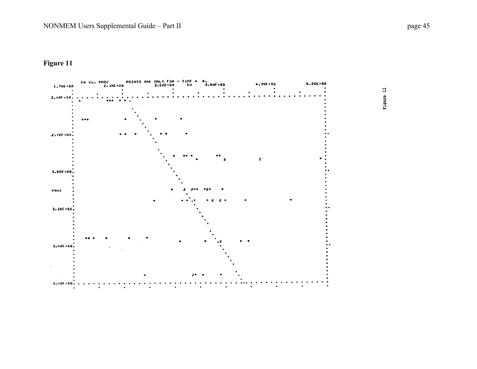
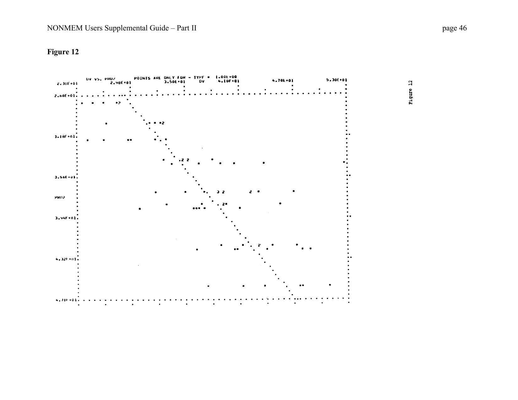
The output from NONMEM from this example is, of course, essentially just that of the old example since only the data set before problem initialization is different, but at problem initialization the data set is transgenerated to look like the old data set. Scatterplots of observed clearance versus predicted clearance and of observed volume versus predicted volume were added to the output in this example and are given in Figure 3, Figure 4. Note the inclusion of the unit slope line (see section C.5).
There are two other values that may be assumed by MODE. If the user only wants to access the data records without modifying them, the value 1 may be used instead of 2. Use of the value 1 will safeguard inadvertent destruction of material in the data set, and it will also save some computing cost. Whatever value is used, 1 or 2, this value must be used on every call to PASS until PASS is reinitialized, with the following exception. If the value 1 is used, then at any call to PASS (after the initializing call) the value 3 may be used, in which case PRED tells PASS that the pass through the data records is to be terminated. A subsequent call to PASS must be an initializing call with MODE set equal to 0.
There are two ways a pass through the data records is terminated. Either the last data record of the data set has already been passed, and PASS returns with MODE equal to 0, or PRED sets MODE equal to 3 and calls PASS. In either case the first data record of the data set is again found in DATREC when PASS returns final control to PRED.
Lastly, during a pass through the data records, the value of the argument NEWIND in PRED changes as it would during a pass through the data records when ICALL is 2.
The possible values of MODE are summarized in Table 1.
| Argument | Value | Function |
|---|---|---|
| MODE | 0 | initialize PASS |
| 1 | obtain next data record; it will not be modified | |
| 2 | obtain next data record; it may be modified | |
| 3 | terminate PASS (used only after MODE=1) |
2.3 FINISH Record
One way to communicate the number of data records to NONMEM is to include this number in field 3 of the DATA control record. Another way is to simply place a blank or zero in that field and place a FINISH record after the last FORTRAN record in the input data file. The FINISH record is regarded as part of the input data file per se, rather than as another control record. Its format is quite simple, though quite different from that of the control records, and is given by the following two rules.
- The FINISH record contains blank characters in positions 1–76 and 80 and the characters F, I and N in positions 77, 78 and 79, respectively.
- If m is the number of FORTRAN records spanned per data record, there must be m–1 blank FORTRAN records inserted before the FINISH record.
In addition, for one to be able to use the FINISH record the following three rules must be followed.
- All FORTRAN records of the input data file must be 80 characters long.
- All FORTRAN records of the input data file except the FINISH record must have blank characters in positions 77–80.
- The total number of A, B and F codes on the FORMAT record, including their multiplicities, must equal, i.e. not exceed, the number of data items specified on the DATA record.
The first of these three rules is always satisfied when the input data file is embedded in the control stream.
Use of the FINISH record is illustrated in Figure 2. The summary of the problem specification for this example is shown in Figure 5. There it may be seen that NONMEM has counted the number of data records and recorded this number on the summary.
The necessary change in the DATA record that accompanies the use of the FINISH record is reflected in the format for this record given in Table 2.
| Field No. | Value | Function |
|---|---|---|
| 1 | 0 or blank | data set embedded in the control stream |
| 1 | between 20 & 99 | FORTRAN unit number for data file |
| 2 | 0 or blank | FORTRAN unit not to be rewound |
| 2 | 1 | FORTRAN unit to be rewound |
| 3 | 0 or blank | FINISH record used |
| 3 | positive integer | number of data records |
| 4 | between 1 & 20 | number of data items per data record |
2.4 Label Option
From Figure 5 it may be noted that the label of the prediction data item is PRD1, rather than the standard label, PRED. Nonstandard labeling for any one of the three data items: prediction, residual and weighted residual data items, is in general accomplished by including user-chosen labels for all three data items on the LABEL record. These three labels follow the labels that generally occur on the LABEL record. In addition, a one is placed in field 6 of the ITEM record. See Figure 2 for illustration. There the user-chosen labels for the residual and weighted residual data items coincide with the standard labels. (Nonstandard labeling, as described here, is not available in NONMEM version I.) The format for the ITEM record, showing the six fields so far defined, is given in Table 3.
| Field no. | Value | Function |
|---|---|---|
| 1 | between 0 & 20 | index of ID data item |
| 2 | between 1 & 20 | index of DV data item |
| 3 | between 0 & 20 | index of MDV data item |
| 4 | between 0 & 20 | number of data item indices in INDXS |
| 5 | 0 or blank | no user data item labels supplied |
| 5 | 1 | user data item labels supplied |
| 6 | 0 or blank | standard labels PRED, RES, WRES used |
| 6 | 1 | nonstandard labels used |
2.5 COVARIANCE Record
There are two matrices that are computed in the Covariance Step as intermediate steps toward computing the covariance matrix. The first matrix, the R matrix, is the Hessian matrix (or second derivative matrix) of the objective function, evaluated at the final estimate of the model parameter (θ, Ω, Σ). The second matrix, the S matrix, is the sum of matrices, \(S_j\), one matrix for each individual. Each matrix, \(S_j\), is \(\nabla_j \nabla_j'\), where \(\nabla_j\) is the gradient (column) vector of the contribution to the objective function from the jth individual, evaluated at the final estimate of the model parameter. Under the assumption that all random effects are normally distributed, the R and S matrices, each divided by the number, N, of individuals in the sample, tend to the same matrix as N increases. In this case the inverse of either matrix serves as an estimate of the true covariance matrix. When the normality assumption is not made, the matrix \(R^{-1} S R^{-1}\) estimates the true covariance matrix. This is the default estimate in NONMEM.
The user may specify that the covariance matrix be given by \(R^{-1}\) or \(S^{-1}\). (This feature is not available in NONMEM Version I, but in Version I the R and/or S matrices may be printed; see below.) In the first case, the standard errors are based on \(R^{-1}\), the inverse covariance matrix is given by R, the correlation matrix is that of \(R^{-1}\), and the eigenvalues (see Section 11.2.6) are those of \(R^{-1}\). Similarly in the second case. To specify that the covariance matrix be given by \(R^{-1}\), a one is placed in field 2 of the COVARIANCE record. To specify that the covariance matrix be given by \(S^{-1}\), a two is placed in this field. To use the default covariance matrix, a blank or zero is placed in this field. (In NONMEM Version I, field 2 is used for a different purpose; see below.)
Suppose the default covariance matrix is used. Then either the R or S matrix, or both matrices, may be printed at the user’s option. To specify that the R matrix, but not the S matrix, be printed, a one is placed in field 3 of the COVARIANCE record. To specify that the S matrix, but not the R matrix be printed, a two is placed in this field. To specify that both R and S be printed, a 3 is placed in this field. The problem specification in Figure 2 specifies that both matrices are to be printed. The desired printout is given in Figure 6, Figure 1.
If a blank or zero is placed in field 3, neither the R nor S matrix is printed (as long as there is also a blank or zero in field 2). Users of NONMEM Version I should use field 2 for the purpose of specifying printing of the R and/or S matrix, rather than field 3.
For a summary of the COVARIANCE record format see the next section.
2.6 Eigenvalues
Another statistic may be output at the user’s option. This is the vector of eigenvalues of the correlation matrix. The individual eigenvalues are ordered from the least in value to the largest in value. To obtain the eigenvalues, a one is placed in field 4 of the COVARIANCE record. See Figure 2 for illustration. The eigenvalues for the example are given in Figure 8. The complete format of the COVARIANCE record is given in Table 4.
| Field no. | Value | Function |
|---|---|---|
| 1 | 0 or blank | Covariance Step conditionally implemented |
| 1 | 1 | Covariance Step unconditionally implemented |
| 1 | 2 | Covariance Step omitted |
| If the value is 2, the subsequent fields may be ignored. | ||
| 2 | 0 or blank | covariance matrix set equal to \(R^{-1} S R^{-1}\) |
| 2 | 1 | covariance matrix set equal to \(R^{-1}\) |
| 2 | 2 | covariance matrix set equal to \(S^{-1}\) |
| 3 | 0 or blank | neither R nor S printed |
| 3 | 1 | R matrix printed |
| 3 | 2 | S matrix printed |
| 3 | 3 | both R and S printed |
| 4 | 0 or blank | eigenvalues not printed |
| 4 | 1 | eigenvalues printed |
Users of NONMEM Version I should use field 3 for the purpose of specifying printing of eigenvalues, rather than field 4.
3 Example Involving Complete Multivariability
3.1 Introduction
In the old example clearance and rate constant of elimination resulting from the same dose were assumed to be statistically independent conditional on the individual to whom the dose was given, i.e. conditional on the values of the first type random effects for the individual. It could not have been otherwise, since it is a property of the general model for one-level nested random effects as described in NONMEM Users Guide, Part I, that the joint levels of the second type random effects are taken to vary between observations and be independent. As a consequence, in the example, sigma was assumed to be diagonal. Since only one of \(\varepsilon_{1ij}\) and \(\varepsilon_{2ij}\) actually affect the observation, \(y_{ij}\), these two random variables cannot be taken to be correlated so long as the above mentioned property of the general model must be satisfied. However, this property actually need not be satisfied, and this is the main idea to be discussed here and in subsequent sections. Let us first extend the model in the old example so that clearance and rate constant of elimination are not taken to be conditionally independent, and sigma is not taken to be diagonal.
Write \(y_{1ij}\) for the CL of the ith pair in the jth individual, and \(y_{2ij}\) for the KE of the ith pair in the jth individual. Also, let \(x_{11ij}\) and \(x_{12ij}\) both be the weight of the jth individual (for all i), and let \(x_{21ij}\) and \(x_{22ij}\) be the numbers 0 and 1, respectively for all i and j. Then let the model for \(y_{rij}\) be given by
\[ \begin{aligned} y_{rij} ={}& f(\theta_1, \theta_2, \theta_3, x_{1rij}, x_{2rij}) \\ &+ g_1(x_{2rij}) \eta_{1j} + g_2(x_{2rij}) \eta_{2j} \\ &+ h_1(x_{2rij}) \varepsilon_{1ij} + h_2(x_{2rij}) \varepsilon_{2ij} \end{aligned} \]
Where
\[ f(\theta_1, \theta_2, \theta_3, x_1, x_2) = \begin{cases} \theta_1 x_1 + \theta_2 & \text{if } x_2 = 0 \\ \theta_3 & \text{if } x_2 = 1 \end{cases} \]
\[g_1(x_2) = \begin{cases} 1 & \text{if } x_2 = 0 \\ 0 & \text{if } x_2 = 1 \end{cases}\]
\[g_2(x_2) = \begin{cases} 1 & \text{if } x_2 = 0 \\ 0 & \text{if } x_2 = 1 \end{cases}\]
\[h_k(x_2) = g_k(x_2) \quad k = 1, 2\]
\[E(\eta_{1j}, \eta_{2j}) = 0 \quad \mathrm{Cov}(\eta_{1j}, \eta_{2j}) = \Omega \quad \text{for all } j\]
\[E(\varepsilon_{1ij}, \varepsilon_{2ij}) = 0 \quad \mathrm{Cov}(\varepsilon_{1ij}, \varepsilon_{2ij}) = \Sigma \quad \text{for all } i, j.\]
There are several differences between this model formulation and the old one. First, and least important, the argument lists for the g and h functions have been shortened since these functions never really depended on those arguments that have been deleted. Second, the second type random effects do not assume different values with different observations; they may assume different values with different pairs of observations. This is why the observations have been triply subscripted, whereas before they were doubly subscripted. However, it is still assumed that the different joint levels of the second type random effects, i.e. the vectors \((\varepsilon_{1ij}, \varepsilon_{2ij})\) for all i and j, are statistically independent. As a result of this difference in the model formulation, \(y_{1ij}\) and \(y_{2ij}\) are certainly not conditionally independent. Third, sigma is not constrained to be diagonal. It need not be, since, although only \(\varepsilon_{1ij}\) affects \(y_{1ij}\) and only \(\varepsilon_{2ij}\) affects \(y_{2ij}\), as just observed \(y_{1ij}\) and \(y_{2ij}\) are not conditionally independent.
This model is but an example of a more general one that may indeed be implemented with NONMEM, and this general model is described in the next section, Section 11.3.2. To use a triply subscripted model, the so-called level two data item must be used, and this is discussed and illustrated for the example in Section 11.3.3.
3.2 The General Model with One-Level Nested Random Effects
The complete form of the general model with one-level nested effects that is implemented in NONMEM is given in this section. The special case, given in section F.5 of the NONMEM Users Guide, Part I, is still quite general and should suffice for most purposes.
The observations are triply subscripted: \(y_{rij}\), r = 1, \(m_{ij}\), i = 1, \(n_j\), j = 1, J where for some j, \(n_j > 1\) and for some i, j, \(m_{ij} > 1\). The model for \(y_{rij}\) is given by
\[y_{rij} = f_{rij}(\theta) + \sum_{k=1}^{K} g_{krij}(\theta) \eta_{kj} + \sum_{l=1}^{L} h_{lrij}(\theta) \varepsilon_{lij}\]
\[E(\eta_{1j}, \eta_{2j}, \ldots, \eta_{Kj}) = 0 \quad \text{for all } j\]
\[\mathrm{Cov}(\eta_{1j}, \eta_{2j}, \ldots, \eta_{Kj}) = \Omega\]
\[E(\varepsilon_{1ij}, \varepsilon_{2ij} \ldots \varepsilon_{Lij}) = 0 \quad \text{for all } i, j\]
\[\mathrm{Cov}(\varepsilon_{1ij}, \varepsilon_{2ij} \ldots \varepsilon_{Lij}) = \Sigma\]
where the \(f_{rij}\), \(g_{krij}\), and \(h_{lrij}\) are functions of the vector-valued parameter, θ, the vectors \(\eta_j = (\eta_{1j}, \eta_{2j}, \ldots, \eta_{Kj})\) are independent random vectors, the vectors \(\varepsilon_{ij} = (\varepsilon_{1ij}, \varepsilon_{2ij} \ldots \varepsilon_{Lij})\) are independent random vectors, and for each i, j, the covariance of \(\eta_j\) and \(\varepsilon_{ij}\) is zero. The triple subscripting on the function f, and on the functions \(g_k\) and \(h_l\), serves as a shorthand alternative to listing the values of the x’s as was done in the example. This model looks very similar to the one in NONMEM Users Guide, Part I. Formally, the only difference appears to be the use of triple, rather than double, subscripting. But this difference is nonetheless the important distinction to be made here and is related to the full multivariate character of observations from a given individual, conditional on the individual.
For θ, and r, i, j, the values of \(g_{1rij}(\theta), g_{2rij}(\theta), \ldots g_{Krij}(\theta)\) are returned in PRED in G(1), G(2), …, G(K), respectively, and the values of \(h_{1rij}(\theta), h_{2rij}(\theta), \ldots h_{Lrij}(\theta)\) are returned by PRED in H(1), H(2), …, H(L) respectively. Both K and L can be at most 5.
The (default) objective function for this model is
\[ O(\theta, \Omega, \Sigma) = \sum_{j=1}^{J} \left[ \log \det C_j(\theta, \Omega, \Sigma) + R_j(\theta, \Omega, \Sigma) R_j'(\theta, \Omega, \Sigma) \right] \]
where
\[y_j = (y_{11j}, y_{21j}, \ldots, y_{m_{n_j 1 j}}, \ldots, Y_{y m_{n_j} n_j j})\]
\[C_j(\theta, \Omega, \Sigma) = \text{covariance matrix of } y_j \text{ under the model}\]
\[f_j(\theta) = (f_{11j}(\theta), f_{21j}(\theta), \ldots, f_{m_{n_j 1 j}}(\theta), \ldots, f_{m_{n_j} n_j j}(\theta))\]
\[R_j(\theta, \Omega, \Sigma) = (Y_j - f_j(\theta)) C_j(\theta, \Omega, \Sigma)^{-1/2}.\]
Now let
\[g_{kj}(\theta) = (g_{k11j}(\theta), g_{k21j}(\theta), \ldots, g_{km_{n_j 1 j}}(\theta), \ldots g_{km_{n_j} n_j j}(\theta))\]
and
\[h_{lj}(\theta) = (h_{l11j}(\theta), h_{l21j}(\theta), \ldots, h_{lm_{n_j 1 j}}(\theta), \ldots, h_{lm_{n_j} n_j j}(\theta))\]
Let \(G_j(\theta)\) be the K by \(Q_j\) matrix whose kth row is \(g_{kj}(\theta)\), and let \(H_j(\theta)\) be the L by \(Q_j\) matrix whose lth row is \(h_{lj}(\theta)\). Here
\[Q_j = m_{1j} + m_{2j} + \ldots + m_{n_j j}.\]
The matrix \(C_j\) can be expressed in terms of the matrices \(G_j\) and \(H_j\). To do this some further notation is needed.
Let Q be a positive integer, and let there be a vector of positive integers, \(q = (q_1, q_2, \ldots q_n)\), whose sum is Q. Let \(A = (a_{ij})\) be a Q-dimensional matrix. Define \(\mathrm{diag}_q A\) to be the block diagonal matrix
\[\begin{pmatrix} A_1 & & & 0 \\ & \ddots & & \\ & & \ddots & \\ 0 & & & A_n \end{pmatrix}\]
Where \(A_k\) is the submatrix of A consisting of those elements \(a_{ij}\) such that
\[\sum_{l=1}^{k-1} q_l < i, j < \sum_{l=1}^{k} q_l.\]
Using this notation, we have
\[C_j(\theta, \Omega, \Sigma) = G_j'(\theta) \Omega G_j(\theta) + \mathrm{diag}_{q_j}(H_j'(\theta) \Sigma H_j(\theta))\]
where \(q_j = (m_{1j}, m_{2j}, \ldots, m_{n_j j})\).
3.3 The Level Two Data Item
To use the triply subscripted model the groups of observations in which the second type random effects do not vary must be delineated for NONMEM. This is done analogously to the way the groups of observations in which the first type random effects do not vary are delineated. That is, a data item like the ID data item is used. One might also call the first type of random effects, level one random effects and the second type of random effects, level two random effects. (There are two levels of random effects, but there is only one level of nesting.) Then the ID data item might be also called the level one (L1) data item, since it is used to group observations according to level one random effects. The data item to be described in this section is called the level two (L2) data item since it is used to group observations according to level two random effects.
In the general model the dependent observations are partitioned into groups in which the level two effects do not vary. These groups are called level two units. In NONMEM the data records whose DV data items are those of a given level two unit may be grouped together, and this is accomplished in part by including in each data record an L2 data item identifying the level two unit containing the DV data item in the record. The L2 data items need not be integer valued (in contrast to the ID data items). A problem specification for the example is given in Figure 2. There the fifth data item of each data record is a L2 data item. Grouping is effected by including the L2 data items in the data records and by arranging that all data records with the same L2 data item be contiguous. The data records with the same L2 data item are collectively called a level two unit record. As with L1 data items, the same L2 data item may actually be used to identify different level two unit records, providing these records are not contiguous in the data set. Level two unit records may consist of one or more case records (see section B.1, NONMEM Users Guide, Part I). Only the last data record of a case record need contain an L2 data item. Obviously, a level two unit record should be contained in a single individual record.
Lastly, the index of the L2 data items should be placed in field 7 of the ITEM record. See Figure 2 for illustration. The complete format of the ITEM record is given in Table 5.
| Field no. | Value | Function |
|---|---|---|
| 1 | between 0 & 20 | index of ID data item |
| 2 | between 1 & 20 | index of DV data item |
| 3 | between 0 & 20 | index of MDV data item |
| 4 | between 0 & 20 | number of data item indices in INDXS |
| 5 | 0 or blank | no. user data item labels supplied |
| 5 | 1 | user data item labels supplied |
| 6 | 0 or blank | standard labels PRED, RES, WRES used |
| 6 | 1 | nonstandard labels used |
| 7 | between 0 & 20 | index of L2 data item |
Users of NONMEM Version I should use field 6 of the ITEM record for the purpose of specifying the presence of L2 data items. (This feature is not available in NONMEM Version I Level 1.)
The code for PRED for the example remains unchanged. In addition to inclusion of L2 data items, the other important difference in the problem specification from that of the old example is the inclusion of an initial estimate for the off-diagonal element of sigma. The initial estimate of sigma (as a matrix) is obtained by first obtaining from each individual an estimate of the covariance matrix of his CL and KE in the usual way. Then these individual estimates are averaged to obtain an estimate, which after being rounded to the first significant figure, serves as the initial estimate of sigma.
There is little difference between the final estimate, as given in Figure 10, and that of the old example. The estimated intraindividual correlation between CL and KE, though, is .54. The standard error of the final estimate is given in Figure 11, and the standard error of the estimate of the intraindividual covariance between CL and KE, in particular, supports the significance of the correlation.
4 Example Involving Utilities CHOL and MULT
4.1 Introduction
In Section 11.2, a NONMEM utility subroutine, PASS, is described. This subroutine can be called by PRED. In this section two other NONMEM utility subroutines that can be called by PRED are described.
The first utility, CHOL, allows the Cholesky square root of a positive definite matrix to be obtained in a convenient way. (CHOL is not available with NONMEM Version I Level 1.) The second utility, MULT, allows the two terms
\[\log \det C_j(\theta, \Omega, \Sigma) \quad \text{and} \quad R_j(\theta, \Omega, \Sigma) R_j'(\theta, \Omega, \Sigma)\]
occurring in the (default) objective function to be weighted unequally, where the weights are computed in PRED and may vary with j. MULT can also be used with CRIT (see Section 10.6). (MULT is not available with NONMEM Version I.) These utilities may be used for a number of different reasons. However, with this example we illustrate only one way in which they may be used. The theoretical aspects of the example are given below. CHOL is described in Section 11.4.2, and MULT is described in Section 11.4.3. The user may wish to go directly to these sections to obtain these descriptions and skip the example.
Consider again the data used in the example of Section 11.3 and the model for this data developed there. For each j, estimates of the three quantities
\[CL_j = \theta_1 w_j + \eta_{1j}\]
\[KE_j = \theta_3 + \eta_{2j}\]
and Σ, where \(w_j\) is the weight of the jth subject, may be obtained from just the 12 observations in the jth subject. \(\hat{CL}_j\) is given by the sample mean of the 6 clearances: \(\hat{KE}_j\) is given by the sample mean of the 6 rate constants: \(\hat{\Sigma}\) is given by the sample covariance matrix of the 6 pairs of clearance and rate constant. Write \(\hat{\Sigma}_j\), instead of \(\hat{\Sigma}\), to indicate that the estimate is based only on the observations from the jth subject. Now assume that the second type random effects are normally distributed. Let m = 6. Then conditional on \(\eta_{1j}\) and \(\eta_{2j}\), \((\hat{CL}_j, \hat{KE}_j)\) is multivariate normally distributed with mean \((CL_j, KE_j)\) and covariance Σ/m, while \((m-1) \hat{\Sigma}_j\) is independently Wishart distributed with parameters Σ and m-1 (2). So unconditionally, \((\hat{CL}_j, \hat{KE}_j)\) is multivariate normally distributed with mean \((\theta_1 w_j, \theta_3)\) and covariance \(\Omega + \Sigma/m\), while \((m-1) \hat{\Sigma}_j\) is independently Wishart distributed with parameters Σ and m-1. Therefore, the negative log-likelihood of \((\theta, \Omega, \Sigma)\) based on the \(\hat{CL}_j, \hat{KE}_j\), and \(\hat{\Sigma}_j\) may be written in a straight forward manner and is the sum of two components, one component, \(S_{1j}\), being the contribution from \((\hat{CL}_j, \hat{KE}_j)\) and the other component, \(S_{2j}\), being the contribution from \(\hat{\Sigma}_j\). The negative log likelihood of \((\theta, \Omega, \Sigma)\) based on \(\hat{CL}_j, \hat{KE}_j\) and \(\hat{\Sigma}_j\) for all j, is of course the sum of \(S_{1j} + S_{2j}\) over all j. We shall indicate how NONMEM may be used to obtain the maximum likelihood estimate of \((\theta, \Omega, \Sigma)\) from the \(\hat{CL}_j, \hat{KE}_j\), and \(\hat{\Sigma}_j\). It may be shown that theoretically this estimate coincides with the estimate obtained in Section 11.3, and that estimate is consistent even though it is developed without the above normality assumption on the second type random effects.
The first component, \(S_{1j}\), is
\[\log \det C_j + ((y_j - f_j) C_j^{-1} (y_j - f_j)')\]
Up to an additive constant, where
\[C_j = \Omega + \Sigma / m\]
\[y_j = (y_{1j}, y_{2j}) \quad y_{1j} = \hat{CL}_j \quad y_{2j} = \hat{KE}_j\]
\[f_j = (f_{1j}, f_{2j}) \quad f_{1j} = \theta_1 w_j \quad f_{2j} = \theta_3\]
This has the form of a term of the NONMEM (default) objective function for a model with equivalently nested random effects (see section D.6 of NONMEM users Guide, Part I). In fact, with appropriate definitions for the functions \(g_{kij}\) and the omega matrix, in NONMEM an individual can be specified whose observations and predictions are \(y_j\) and \(f_j\) and whose \(C_j\) is \(\Omega + \Sigma/m\). Define the omega matrix to be the block diagonal matrix
\[\begin{pmatrix} \Omega & 0 \\ 0 & \Sigma \end{pmatrix}\]
(use the constraint on omega described in section B). Define
\[g_{1ij} = \begin{cases} 1 & \text{if } i = 1 \\ 0 & \text{otherwise} \end{cases}\]
\[g_{2ij} = \begin{cases} 1 & \text{if } i = 2 \\ 0 & \text{otherwise} \end{cases}\]
\[g_{3ij} = \begin{cases} C & \text{if } i = 1 \\ 0 & \text{otherwise} \end{cases}\]
\[g_{4ij} = \begin{cases} C & \text{if } i = 2 \\ 0 & \text{otherwise} \end{cases}\]
where \(c = 1/\sqrt{6}\). That is, \(G_j'\) is
\[\begin{pmatrix} 1 & 0 & C & 0 \\ 0 & 1 & 0 & C \end{pmatrix}\]
The second component, \(S_{2j}\), is
\[(m-1) \log \det \Sigma + (m-1) \mathrm{tr}(\hat{\Sigma}_j \Sigma^{-1})\]
up to an additive constant. Since \(\hat{\Sigma}_j\) is positive definite, there exists a 2-dimensional lower triangular matrix \(T_j\) such that \(T_j T_j' = \hat{\Sigma}_j\). This matrix is called the Cholesky square root of \(\hat{\Sigma}_j\). Since
\[\mathrm{tr}(\hat{\Sigma}_j \Sigma^{-1}) = \mathrm{tr}(T_j \Sigma^{-1} T_j'),\]
the second component may be written as the sum of two terms:
\[((m-1)/2) \log \det \Sigma + (m-1) T_{jr} \Sigma^{-1} T_{jr}' \quad r = 1, 2\]
where \(T_{jr}\) is the rth row of \(T_j\). The rth term may in turn be written as
\[((m-1)/2) \log \det C_j + (m-1)(y_j - f_j) C_j^{-1} (y_j - f_j)'\]
where now
\[C_j = \Sigma \quad y_j = T_{jr} \quad f_j = 0.\]
Momentarily ignoring the two coefficients \((m-1)/2\) and \(m-1\), this again has the form of a term of the NONMEM (default) objective function for a model with equivalently nested random effects. With appropriate definitions for the functions \(g_{kij}\) and with the same block diagonal omega matrix as given above, in NONMEM an individual can be specified whose observations and predictions are \(y_j\) and \(f_j\) and whose \(C_j\) is Σ. Define
\[g_{1ij} = 0 \quad \text{for } i = 1, 2\]
\[g_{2ij} = 0 \quad \text{for } i = 1, 2\]
\[g_{3ij} = \begin{cases} 1 & \text{if } i = 1 \\ 0 & \text{if } i = 2 \end{cases}\]
\[g_{4ij} = \begin{cases} 0 & \text{if } i = 1 \\ 1 & \text{if } i = 2 \end{cases}\]
That is, \(G_j'\) is
\[\begin{pmatrix} 0 & 0 & 1 & 0 \\ 0 & 0 & 0 & 1 \end{pmatrix}\]
Hence, three individuals may be specified, each of which contributes a term to the NONMEM objective function, and the sum of these three terms is \(S_{1j} + S_{2j}\). Thus NONMEM may be used to obtain the desired maximum likelihood estimate. There remain, though, two problems. The first is that of obtaining the \(T_{jr}\), and the second is that of introducing the coefficients, \((m-1)/2\) and \(m-1\), into the objective function where this is necessary. Solutions to these problems are presented in the next two sections.
4.2 Cholesky Square Root (CHOL)
CHOL is a NONMEM utility subroutine that may be called by PRED. It computes the Cholesky square root of a given positive definite matrix A, i.e. the lower triangular matrix B satisfying BB’=A. (It is not available with NONMEM Version I Level 1.) It is used in a fashion that is particularly convenient for PRED. If the dimension of A is n, then CHOL is called n+1 times in succession. The first call initializes the routine. On the (i+1)st call, the ith row of A is passed to CHOL, and CHOL returns the ith row of B (i=1,…,n). Now suppose A is stored in the data set with the elements of each row of A stored as data items of some data record, a different data record for each row. Until each of the involved data records is passed to PRED, the entire matrix A cannot be made available to PRED. Nonetheless, due to the way in which CHOL is organized (as just described), as each data record is passed to PRED a different row of B can be made available to PRED.
There are four arguments in the subroutine’s argument list. The first argument should be set by PRED to the integer 0 or 1 according to whether the call to CHOL is the initialization call or not. The second argument should be set to the (integer) dimension of A. The third argument should be set to the ith row vector of A on the (i+1)st call to CHOL. (The elements \(a_{ij}\), j>i, are ignored.) Upon return to PRED, the ith row vector of B is found in the third argument. (The elements \(b_{ij}\), j>i, are all zero.) The fourth argument contains an integer return code from CHOL each time a return occurs. Upon return from the initialization call, this code is always 0. Upon return from the (i+1)st call, this code is 0 unless CHOL has determined that based on the first i rows of A, A is algorithmically not positive definite, in which case the return code is 1. At the initialization call, the fourth argument should be set by PRED to either 0 or 1. If it is set to 0 at subroutine initialization, then whenever CHOL is about to return with a return code of 1, CHOL actually terminates NONMEM execution and prints an appropriate message (so the return never really occurs). If the fourth argument is set to 1 at subroutine initialization, then CHOL always returns control to PRED along with the appropriate return code. These arguments are summarized in Table 6.
| Argument | Value | Function |
|---|---|---|
| MODE | 0 or blank | initialize CHOL |
| MODE | 1 | a matrix row is being passed |
| N | between 1 & 5 | dimension of matrix |
| R | row of matrix | |
| IER | upon input when MODE is 0: | |
| 0 | CHOL terminates execution if matrix is algorithmically not positive definite | |
| 1 | CHOL will always return control to PRED |
|
| upon output: | ||
| 0 | normal return | |
| 1 | matrix is algorithmically not positive definite |
For the example, the code for PRED is shown in Figure 12, and the problem specification is shown in Figure 13. Look first at the input data file. The data records are arranged in 12 groups of six data records each. (Each data record of a particular group has the same first digit in its ID data item.) The DV data item of the first data record of the jth group is \(\hat{CL}_j\), and the DV data item of the second data record of the jth group is \(\hat{KE}_j\). The DV data items of the remaining 4 data records of the jth group are all zero. However, the fifth data item of the third data record of the jth group is the first element of the first row of \(\hat{\Sigma}_j\), and the fifth and sixth data items of the fifth data record of the jth group are the first and second elements of the second row of \(\hat{\Sigma}_j\). Therefore, the rows of \(T_j\) may be obtained. This is accomplished by using CHOL during the problem initialization phase of PRED, so that these rows may be stored as DV data items to be used by NONMEM during problem execution. (See the discussion below about the PRED code.) The first and second elements of \(T_{j1}\) may be obtained from the third data record of the jth group, and these elements are to be stored as the DV data items of the third and fourth data records, respectively. The first and second elements of \(T_{j2}\) may be obtained from the fifth data record of the jth group, and these elements are to be stored as the DV data items of the fifth and sixth data records, respectively.
Each of the groups of six data records just described is comprised of three individual records. Consider the jth group. The DV data items of the first individual record are \(\hat{CL}_j\) and \(\hat{KE}_j\). The DV data items of the second individual record are the elements of \(T_{j1}\), and the DV data items of the third individual record are the elements of \(T_{j2}\) (after PRED initialization). These three individual records have the three ID data items j1, j2 and j3, respectively. A type data item also appears in each data record, and this data item takes a unique value for each data record of an individual record so that these different data records may be clearly identified. This is the fourth data item in the data record. The weight data item appears as the second data item in both data records of the first individual record of the jth group.
Notice too that, whereas in the previous examples where clearance has been modeled as a linear function of weight, whose intercept has been constrained to be zero, in this example the intercept has simply been eliminated so that there are only two elements of theta. These are the slope parameter of the linear function and the population mean elimination rate constant. Omega is constrained to be block diagonal with two blocks, each of dimension 2. Notice the use of the structure and BLOCK SET records to accomplish this (see section B).
Regarding next the code for PRED, it may be seen that there are three different pieces of code, starting at statements 5, 10 and 25, only one of which is executed during any particular call to PRED, depending on the value of ICALL. During problem initialization, i.e. when ICALL is 1, CHOL is used to obtain the \(T_j\), as mentioned above. This task is embedded in a pass through the data set using the NONMEM utility PASS (see Section 11.2.2). For each j, the 6 data records of the jth group are successively passed to PRED. The first two data records are simply ignored. Then CHOL is initialized. Then during the first of the two executions of the DO loop, CHOL is used to obtain the elements of \(T_{j1}\) from the information on the third data record, and these elements are stored as the DV data items of the third and fourth data records. During the second execution of the DO loop, CHOL is used to obtain the elements of \(T_{j2}\) from the information on the fifth data record, and these elements are stored as the DV data items of the fifth and sixth data records. When ICALL is 2, F and G are computed according to the discussion in Section 11.4.1. See the next section for the explanation of the call to MULT.
4.3 Reweighting Objective Function (MULT)
The (default) NONMEM objective function is the sum of terms
\[A_j \log \det C_j(\theta, \Omega, \Sigma) + B_j R_j(\theta, \Omega, \Sigma) R_j'(\theta, \Omega, \Sigma)\]
over all j, where all \(A_j\) and \(B_j\) are equal to 1. Other values of \(A_j\) and \(B_j\) may be used. The NONMEM utility subroutine MULT allows these quantities to be set by PRED to values other than 1. (This feature is not available in NONMEM Version I.) To set \(A_j\) and \(B_j\) to a and b, say, PRED issues a single call to MULT during any one or more calls to it from NONMEM where i) ICALL is 2 and ii) some data record from the jth individual record is in DATREC. (At least one such call to MULT must be issued while ICALL is 2, and data records from the jth individual record are being passed to PRED in DATREC.) MULT has only two arguments; the first is set to a and the second to b. (If during each of a number of calls to PRED while i and ii hold, MULT is called, then each time MULT is called it should be called with the same values for its two arguments.)
In Section 10.6 it is explained that the contribution to the objective function from the jth individual may be taken to be
\[A_j \log \det C_j(\theta, \Omega, \Sigma) + B_j \varphi_j(R_j(\theta, \Omega, \Sigma))\]
where \(A_j\) and \(B_j\) are equal to 1 and \(\varphi_j\) is some function of the vector of weighted residuals from the jth individual other than the inner product. MULT can be used, as described above, to allow PRED to set \(A_j\) and \(B_j\) to values other than 1.
In the code for PRED in the example, given in Figure 12, it may be seen that with every individual record with ID data item ending in 2 or 3, MULT is called with arguments equal to \((m-1)/2\) and \(m-1\) whenever the last data record of the individual record is in DATREC.
Figures
      SUBROUTINE PRED (ICALL,NEWIND,THETA,DATREC,INDXS,F,G,H)
C
C     THETA(1)=CLEARANCE SLOPE(LITERS/HR/KG)
C     THETA(2)=CLEARANCE INTERCEPT(LITERS/HR)
C     THETA(3)=KE MEAN(1/HR)
C     DATREC(1)=ID DATA ITEM
C     DATREC(2)=WEIGHT(KG)
C     DATREC(3)=DV DATA ITEM
C                VOLUME(LITERS) IS TRANSGENERATED TO KE(1/HR)
C                AT PROBLEM INITIALIZATION
C                KE(1/HR) IS TRANSGENERATED TO VOLUME(LITERS)
C                AT PROBLEM FINALIZATION
C     DATREC(4)=TYPE DATA ITEM
C     DATREC(5)=PREDICTION DATA ITEM
C                KE(1/HR) IS TRANSGENERATED TO VOLUME(LITERS)
C
      DIMENSION THETA(1),DATREC(1),INDXS(1),G(1),H(1)
      K=ICALL+1
      GO TO (5,10,20,25), K
    5 RETURN
   10 MODE=0
      CALL PASS (MODE)
      MODE=2
   15 CALL PASS (MODE)
      IF (MODE.EQ.0) RETURN
      M=DATREC(4)
      IF (M.EQ.0) A=DATREC(3)
      IF (M.EQ.1) DATREC(3)=A/DATREC(3)
      GO TO 15
   20 F=(THETA(1)*DATREC(2)+THETA(2))*(1.0-DATREC(4))+THETA(3)*DATREC(4)
      G(1)=1.0-DATREC(4)
      G(2)=DATREC(4)
      H(1)=1.0-DATREC(4)
      H(2)=DATREC(4)
      RETURN
   25 MODE=0
      CALL PASS (MODE)
      MODE=2
   30 CALL PASS (MODE)
      IF (MODE.EQ.0) RETURN
      M=DATREC(4)
      IF (M.EQ.1) GO TO 35
      B=THETA(1)*DATREC(2)+THETA(2)
      DATREC(5)=B
      A=DATREC(3)
      GO TO 30
   35 DATREC(5)=B/THETA(3)
      DATREC(3)=A/DATREC(3)
      GO TO 30
ENDPRED: transgeneration example. Re-typeset from the original dot-matrix scan for legibility.
PROB    MULTIV LIN REGRESSION OF CL AND KE VS WT WITH VARIANCE COMPONENTS
DATA       0    0    0    5
ITEM       1    3    0    0    1    1
LABL       ID       WT       DV       TYPE     PRD2     PRD1     RES      WRES
FORM
(F2.0,1X,F4.0,1X,F6.0,1X,F1.0,1X,F1.0)
 1 79.6   1.850 0
 1 79.6  38.947 1
 1 79.6   2.642 0
 1 79.6  47.348 1
 1 79.6   1.963 0
 1 79.6  44.614 1
 1 79.6   2.415 0
 1 79.6  43.125 1
 1 79.6   1.905 0
 1 79.6  43.100 1
 1 79.6   2.120 0
 1 79.6  41.326 1
 2 72.4   3.270 0
 2 72.4  32.831 1
 ... [remaining data records elided — 144 records total; 12 records per individual for 12 individuals; see scanned figures 10a–10c for full listing] ...
12 60.5   2.406 0
12 60.5  32.959 1
                                                                             FIN
STRC       3    2    2    1    0    0    1    1
STRC       1    2
THTA     .04     0.0     .08
LOWR     0.      0.      0.0
UPPR   +10000000.0    +1000000.0    +1000000
BLST     .4     .006     .0002
DIAG     .1             .00008
ESTM       0  300    3    5
COVR       0    0    3    1
TABL       0    1
TABL       4    1    2    2    0    4    1    5    0
SCAT       0    4
SCAT       5    3    1    4    0    1
SCAT       2    4
SCAT       2    8    1    4
SCAT 2 7 1 4PRED. The FIN marker denotes the FINISH record (cols 77–79) used because field 3 of the DATA record is blank (see Section 11.2.3). Full 144-record data listing elided for readability; see the scanned figure for the complete listing.
NONLINEAR MIXED EFFECTS MODEL PROGRAM (NONMEM)    VERSION 2 LEVEL 1    CDC=6600 VERSION
DEVELOPED AND PROGRAMMED BY STUART BEAL AND LEWIS SHEINER

PROBLEM NO.  1
MULTIV LIN REGRESSION OF CL AND KE VS WT WITH VARIANCE COMPONENTS

DATA SET IDENTICAL TO PREVIOUS DATA SET:       NO
DATA SET IN CONTROL STREAM:             YES
NO. OF DATA ITEMS IN DATA SET:    5
ID DATA ITEM IS DATA ITEM NO.:    1
DEP VARIABLE IS DATA ITEM NO.:    3

LABELS TO BE USED FOR ITEMS APPEARING
    IN TABLES AND SCATTERPLOTS ARE:
ID       WT       DV       TYPE     PRD2     PRD1     RES      WRES

FORMAT FOR DATA IS:
(F2.0,1X,F4.0,1X,F6.0,1X,F1.0,1X,F1.0)

TOT. NO. OF DATA RECS:       144
TOT. NO. OF CASE RECS:       144
TOT. NO. OF INDIVIDUALS:       12

LENGTH OF THETA:   3

OMEGA HAS BLOCK FORM:
 1
 1  1

SIGMA HAS SIMPLE DIAGONAL FORM WITH DIMENSION  2

INITIAL ESTIMATE OF THETA:
LOWER BOUND        INITIAL EST       UPPER BOUND
  0.                0.4000E-01         0.1000E+07
  0.                0.                 0.
  0.                0.8000E-01         0.1000E+07

INITIAL ESTIMATE OF OMEGA:
BLOCK SET NO.   BLOCK                                                       FIXED
      1                                                                      NO
             0.4000E+00
             0.6000E-02   0.2000E-03

INITIAL ESTIMATE OF SIGMA:
 0.1000E+00
 0.                 0.8000E-04

ESTIMATION STEP OMITTED:           NO
NO. OF FUNCT. EVALS. ALLOWED:    300
NO. OF SIG. FIGURES REQUIRED:      3
INTERMEDIATE PRINTOUT:            YES
CONVERGENCE REPEATED:              NO

COVARIANCE STEP OMITTED:           NO
R MATRIX PRINTED:                 YES
S MATRIX PRINTED:                 YES
EIGENVALUES PRINTED:              YES

TABLES STEP OMITTED:               NO
NO. OF TABLES PRINTED:              1

USER CHOSEN DATA ITEMS FOR TABLE  1,
IN THE ORDER THEY WILL APPEAR IN THE TABLE, ARE:
TYPE     ID       WT       PRD2
    THE FIRST 2 OF THESE WILL BE SORTED IN THE ORDER IN WHICH THEY APPEAR

SCATTERPLOT STEP OMITTED:          NO
NO. OF PAIRS OF ITEMS GENERATING
        FAMILIES OF SCATTERPLOTS:   4

ITEMS TO BE SCATTERED ARE:      PRD2     DV
    FOR FIXED VALUES OF ITEMS:    TYPE
    UNIT SLOPE LINE INCLUDED
ITEMS TO BE SCATTERED ARE:      WT       WRES
ITEMS TO BE SCATTERED ARE:      WT       WRES
    FOR FIXED VALUES OF ITEMS:    TYPE
ITEMS TO BE SCATTERED ARE:      WT       RES
FOR FIXED VALUES OF ITEMS: TYPE***********************************...*********************************** *********************
***********************... *********************
*********************** R MATRIX *********************
***********************... *********************
***********************************...*********************************** *********************
TH 1 TH 2 TH 3 OM11 OM12 OM22 SG11 SG12 SG22
TH 1 1.01E+06
TH 2 ......... .........
TH 3 -5.90E+05 ......... 4.22E+05
OM11 -2.13E+02 ......... -8.20E+00 1.70E+03
OM12 -4.99E+04 ......... 8.40E+03 -1.45E+05 1.32E+07
OM22 2.44E+06 ......... -4.22E+05 3.00E+06 -2.90E+00 7.40E+08
SG11 -1.15E+01 ......... 1.90E+01 2.91E+02 -2.41E+04 4.90E+04 1.90E+03
SG12 ......... ......... ......... ......... ......... ......... ......... .........
SG22 4.52E+05 ......... -1.98E+04 4.90E+05 -4.90E+07 1.23E+08 8.34E+04 ......... 3.75E+09......... as printed.
***********************************...***********************************    *********************
***********************...                                                    *********************
***********************                       S MATRIX                        *********************
***********************...                                                    *********************
***********************************...***********************************    *********************

        TH 1       TH 2       TH 3       OM11       OM12       OM22       SG11       SG12       SG22

TH 1    8.04E+05
TH 2   .........  .........
TH 3  -5.40E+03  .........   4.22E+05
OM11   1.10E+04  .........  -1.44E+03   1.90E+03
OM12  -3.00E+05  .........  -2.36E+05  -1.43E+05   1.15E+07
OM22  -4.01E+06  .........   7.70E+05   2.50E+06  -2.25E+00   5.10E+04
SG11   2.23E+04  .........  -1.22E+04   1.25E+03  -7.97E+04   1.20E+00   2.92E+03
SG12   .........  .........  .........  .........  .........  .........  .........  .........
SG22 -2.43E+07 ......... 1.53E+07 7.80E+05 -9.51E+07 2.20E+04 1.30E+06 ......... 6.80E+04......... as printed.
***********************************...***********************************    *********************
***********************...                                                    *********************
***********************               EIGENVALUES OF COR MATRIX OF ESTIMATE    *********************
***********************...                                                    *********************
***********************************...***********************************    *********************

            1           2           3           4           5           6           7
1.38E-03 2.56E-02 7.44E-02 3.03E-01 1.27E+00 1.46E+00 3.86E+00PROB MULTIV LIN REGRESSION OF CL AND KE VS WT WITH VARIANCE COMPONENTS
DATA 0 0 144 5
ITEM 1 3 0 0 1 0 5
LABL ID WT DV TYPE LEV2
FORM
(F2.0,1X,F4.0,1X,F6.0,1X,F1.0,1X,F1.0)
1 79.6 1.850 0 0
1 79.6 0.047 1 0
1 79.6 2.642 0 1
1 79.6 0.056 1 1
1 79.6 1.963 0 0
1 79.6 0.044 1 0
1 79.6 2.415 0 1
1 79.6 0.056 1 1
1 79.6 1.905 0 0
1 79.6 0.044 1 0
1 79.6 2.120 0 1
1 79.6 0.051 1 1
2 72.4 3.270 0 0
2 72.4 0.100 1 0
... [remaining data records elided — 144 records total; see scanned figures 17a–17c for full listing] ...
12 60.5 2.406 0 0
12 60.5 0.073 1 1
STRC 3 2 2 1 0 0 1 1 2
STRC 1 2
THTA .04 0.0 .08
LOWR 0. 0. 0.0
UPPR +10000000.0 +1000000.0 +1000000
BLST .4 .006 .0002
BLST .1 .002 .00008
ESTM 0 500 3 5
COVR 1
TABL 1 1
TABL 3 1 2 2 0 4 1
SCAT 1 3
SCAT 2 8 1 4
SCAT 2 7 1 4***********************************...*********************************** *********************
***********************... *********************
*********************** FINAL PARAMETER ESTIMATE *********************
***********************... *********************
***********************************...*********************************** *********************
THETA - VECTOR OF FIXED EFFECTS *********************
TH 1 TH 2 TH 3
4.46E-02 0. 8.43E-02
OMEGA - COV MATRIX FOR RANDOM EFFECTS - ETAS ********
ETA1 ETA2
ETA1 3.27E-01
ETA2 6.73E-03 1.86E-04
SIGMA - COV MATRIX FOR RANDOM EFFECTS - EPSILONS ****
EPS1 EPS2
EPS1 1.25E-01
EPS2 1.86E-03 9.29E-05************************************************************* ********************
************************* STANDARD ERROR OF ESTIMATE ********************
********************* ********************
****************************
************************************************************************************************
THETA - VECTOR OF FIXED EFFECTS ********************
TH 1 TH 2 TH 3
2.34E-03 ......... 3.78E-03
OMEGA - COV MATRIX FOR RANDOM EFFECTS - ETAS *********
ETA1 ETA2
ETA1 1.62E-01
ETA2 3.74E-03 9.20E-05
SIGMA - COV MATRIX FOR RANDOM EFFECTS - EPSILONS ****
EPS1 EPS2
EPS1 2.65E-02
EPS2 6.33E-04 2.24E-05......... in the THETA row) preserved as printed — they mark fixed or non-estimated parameters.
      SUBROUTINE PRED (ICALL,NEWIND,THETA,DATREC,INDXS,F,G,H)
C
C     THETA(1)=POPULATION CLEARANCE SLOPE(LITERS/HR/KG)
C     THETA(2)=POPULATION KE(1/HR)
C     DATREC(1)=ID DATA ITEM
C     DATREC(2)=WEIGHT(KG)
C     DATREC(3)=DV DATA ITEM
C     DATREC(4)=TYPE DATA ITEM
C     DATREC(5)-DATREC(6)=ELEMENTS OF A ROW OF SIGMA HAT
C
      DIMENSION THETA(1),DATREC(1),INDXS(1),G(1),H(1)
      DIMENSION A(2)
      K=ICALL+1
      GO TO (5,10,25,5), K
    5 RETURN
   10 C=1./SQRT(6.)
      MODE=0
      CALL PASS (MODE)
      MODE=2
   14 CALL PASS (MODE)
   15 IF (MODE.EQ.0) RETURN
      IF (DATREC(4).LE.2.) GO TO 14
      IER=0
      CALL CHOL (0,2,A,IER)
      DO 20 I=1,2
      A(1)=DATREC(5)
      A(2)=DATREC(6)
      CALL CHOL (1,2,A,IER)
      DATREC(3)=A(1)
      CALL PASS (MODE)
      DATREC(3)=A(2)
   20 CALL PASS (MODE)
      GO TO 15
   25 M=DATREC(4)
      IF (M.LE.2) GO TO 30
      F=0.
      G(1)=0.
      G(2)=0.
      G(3)=0.
      G(4)=0.
      G(M)=1.
      IF (M.EQ.4) CALL MULT (2.5,5.)
      RETURN
   30 G(1)=0.
      G(2)=0.
      G(3)=0.
      G(4)=0.
      G(M)=1.
      G(M+2)=C
      IF (M.EQ.2) GO TO 35
      F=DATREC(2)*THETA(1)
      RETURN
   35 F=THETA(2)
      RETURN
ENDPRED: example involving utilities CHOL and MULT. Re-typeset from the original low-resolution scan for legibility.
PROB    MULTIV LIN REG OF CL HAT, KE HAT, AND SIGMA HAT VS WT
DATA       0    0   72    6
ITEM       1    3    0    0    1    1
LABL       ID       WT       DV       TYPE     S1       S2
FORM
(F3.0,1X,F4.0,1X,F6.0,1X,F1.0,2(1X,E11.4))
 11 79.6 0.1492 1
 11 79.6 0.0498 2
 12                3    0.9983E-01
 12                4
 13                3    0.1839E-02   0.2940E-04
 13                4
 21 72.4 3.7592 1
 21 72.4 0.0968 2
 22                3    0.1086E 00
 22                4
 23                3    0.4843E-03   0.1117E-04
 23                4
 31 70.5 3.3200 1
 31 70.5 0.0887 2
 32                3    0.6116E-01
 32                4
 33                3    0.1107E-02   0.1133E-03
 33                4
 41 72.7 3.2713 1
 41 72.7 0.0907 2
 42                3    0.6603E 00
 42                4
 43                3    0.2203E-03   0.1565E-04
 43                4
 51 54.6 2.1625 1
 51 54.6 0.0635 2
 52                3    0.4194E-01
 52                4
 53                3    0.1562E-02   0.0139E-04
 53                4
 61 80.0 3.5900 1
 61 80.0 0.0843 2
 62                3    0.1036E 00
 62                4
 63                3    0.1730E-02   0.1162E-03
 63                4
 71 64.6 3.3037 1
 71 64.6 0.0940 2
 72                3    0.5941E-01
 72                4
 73                3    0.1194E-02   0.4226E-04
 73                4
 81 70.5 3.3062 1
 81 70.5 0.0813 2
 82                3    0.1339E 00
 82                4
 83                3   -0.2366E-04   0.3016E-04
 83                4
 91 86.4 3.2353 1
 91 86.4 0.0729 2
 92                3    0.1085E 00
 92                4
 93                3    0.2425E-02   0.1256E-03
 93                4
101 58.2 2.3123 1
101 58.2 0.0743 2
102                3    0.2974E 00
102                4
103                3    0.8180E-02   0.2524E-03
103                4
111 65.0 3.9815 1
111 65.0 0.0977 2
112                3    0.3190E 00
112                4
113                3   -0.3036E-03   0.4670E-04
113                4
121 60.5 2.7080 1
121 60.5 0.0952 2
122                3    0.1157E 00
122                4
123                3    0.3575E-02   0.2303E-03
123                4
STRC       2    4    0    1    0    0    2
STRC       1    2    1    2
THTA     .04     .08
LOWR     0.0     0.0
UPPR   +1000000+1000000
BLST     .4     .006     .0002
BLST     .1     .002     .00008
ESTM       0  500    3    5
COVR       1
TABL       2
SCAT       2